Excel Functions Cheat Sheet is an incredibly powerful tool used across industries for data analysis, organization, and reporting. One of its most valuable features is the vast array of built-in functions, which allow users to manipulate and analyze data with ease. However, with so many formulas available, it can be overwhelming for both beginners and even seasoned users to remember how and when to use each function.
This cheat sheet aims to break down the most important and commonly used Excel functions, making it easier for you to reference when needed. Whether you are new to Excel or looking to level up your skills, this guide will help you become more proficient in handling data efficiently.
1. Basic Math Functions

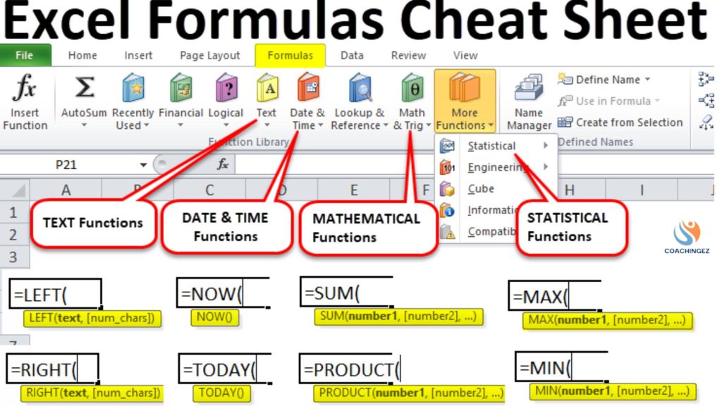
Excel Functions Cheat Sheet
1.1 SUM
The SUM function is one of the simplest and most frequently used formulas in Excel. It allows you to quickly add up values in a range of cells.
Formula:=SUM(A1:A10)
Example:
If cells A1 to A10 contain values, this formula will return their sum.
1.2 AVERAGE
The AVERAGE function calculates the mean (average) of a range of numbers.
Formula:=AVERAGE(A1:A10)
Example:
If A1 to A10 contain numerical values, this function will return their average.
1.3 COUNT
The COUNT function counts the number of cells that contain numerical values within a range.
Formula:=COUNT(A1:A10)
Example:
This formula will return the count of cells that have numbers in them between A1 and A10.
1.4 MIN/MAX
The MIN and MAX functions return the smallest and largest numbers in a range, respectively.
Formula:
=MIN(A1:A10)=MAX(A1:A10)
Example:
The MIN function returns the smallest value, and the MAX function returns the largest value from the selected range.
1.5 ROUND
The ROUND function rounds a number to a specified number of digits.
Formula:=ROUND(A1, 2)
Example:
This rounds the number in A1 to 2 decimal places.
2. Text Functions
2.1 CONCATENATE (or TEXTJOIN in newer versions)
CONCATENATE joins two or more text strings into one.
Formula:=CONCATENATE(A1, B1)
Example:
If A1 contains “Hello” and B1 contains “World,” this formula will return “HelloWorld.”
In newer Excel versions, TEXTJOIN is a more flexible alternative that allows you to specify a delimiter.
Formula:=TEXTJOIN(", ", TRUE, A1, B1)
Example:
Returns “Hello, World.”
2.2 LEFT/RIGHT
LEFT and RIGHT extract a specific number of characters from a string, either from the start (left) or the end (right).
Formula:
=LEFT(A1, 3)=RIGHT(A1, 3)
Example:
If A1 contains “Excel Functions,” LEFT(A1, 5) returns “Excel” and RIGHT(A1, 9) returns “Functions.”
2.3 LEN
LEN returns the length of a text string.
Formula:=LEN(A1)
Example:
If A1 contains “Excel”, LEN(A1) returns 5.
2.4 UPPER/LOWER
UPPER converts a text string to uppercase, while LOWER converts it to lowercase.
Formula:
=UPPER(A1)=LOWER(A1)
Example:
If A1 contains “excel,” UPPER(A1) returns “EXCEL” and LOWER(A1) returns “excel.”
2.5 FIND/SEARCH
FIND and SEARCH locate the position of a specific character or substring within a string.
Formula:=FIND("X", A1)
Example:
If A1 contains “Excel,” this returns the position of “X” (1).
3. Logical Functions
3.1 IF
IF checks whether a condition is met, returning one value if TRUE and another if FALSE.
Formula:=IF(A1 > 10, "Yes", "No")
Example:
If A1 is greater than 10, the function returns “Yes”; otherwise, it returns “No.”
3.2 AND/OR
AND returns TRUE if all conditions are met, while OR returns TRUE if at least one condition is met.
Formula:
=AND(A1 > 10, B1 < 5)=OR(A1 > 10, B1 < 5)
Example:AND returns TRUE if both A1 is greater than 10 and B1 is less than 5. OR returns TRUE if either condition is met.
3.3 NOT
NOT reverses the logical value of its argument.
Formula:=NOT(A1 > 10)
Example:
If A1 is greater than 10, this returns FALSE; otherwise, it returns TRUE.
3.4 IFERROR
IFERROR returns a custom result when a formula generates an error.
Formula:=IFERROR(A1/B1, "Error")
Example:
If B1 is 0 (causing a division error), this formula will return “Error.”
4. Lookup & Reference Functions

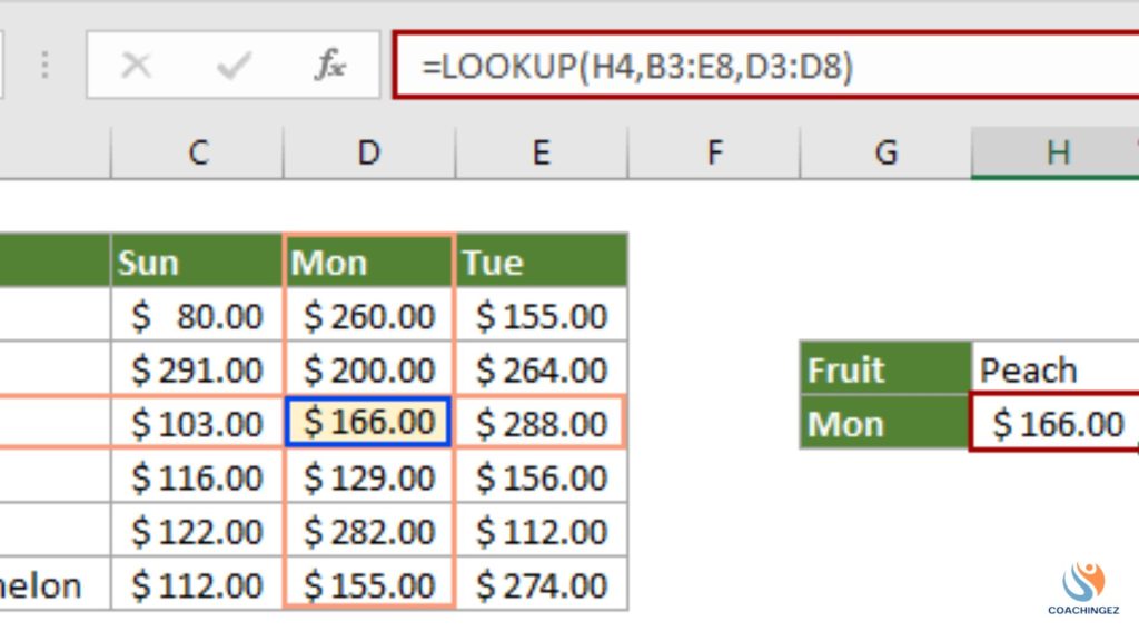
Lookup & Reference Functions
4.1 VLOOKUP
VLOOKUP searches for a value in the first column of a range and returns a value in the same row from a specified column.
Formula:=VLOOKUP(A1, B1:D10, 2, FALSE)
Example:
This looks for the value in A1 within the range B1 and returns the value from the second column.
4.2 HLOOKUP
HLOOKUP works like VLOOKUP, but searches across the first row instead of the first column.
Formula:=HLOOKUP(A1, B1:D10, 2, FALSE)
Example:
Looks across the first row for the value in A1 and returns the value from the second row.
4.3 INDEX
INDEX returns the value at a specific row and column within a range.
Formula:=INDEX(A1:C10, 2, 3)
Example:
Returns the value in the second row and third column of the range A1
.
4.4 MATCH
MATCH returns the relative position of an item in a range that matches a specified value.
Formula:=MATCH(A1, B1:B10, 0)
Example:
Returns the position of the value in A1 within the range B1
.
4.5 INDIRECT
INDIRECT returns the reference specified by a text string.
Formula:=INDIRECT("A" & B1)
Example:
If B1 contains the value 5, this returns the value in cell A5.
5. Date and Time Functions
5.1 TODAY
TODAY returns the current date.
Formula:=TODAY()
Example:
This will return the current date, such as “2024-10-04.”
5.2 NOW
NOW returns the current date and time.
Formula:=NOW()
Example:
Returns the current date and time, like “2024-10-04 12:34.”
5.3 YEAR/MONTH/DAY
YEAR, MONTH, and DAY extract the respective components from a date.
Formula:
=YEAR(A1)=MONTH(A1)=DAY(A1)
Example:
If A1 contains “2024-10-04,” YEAR(A1) returns 2024, MONTH(A1) returns 10, and DAY(A1) returns 4.
5.4 DATEDIF
DATEDIF calculates the difference between two dates.
Formula:=DATEDIF(A1, B1, "d")
Example:
This returns the number of days between the dates in A1 and B1.
5.5 NETWORKDAYS
NETWORKDAYS returns the number of working days between two dates, excluding weekends and holidays.
Formula:=NETWORKDAYS(A1, B1, C1:C5)
Example:
Calculates the number of working days between A1 and B1, considering holidays in C1
.
6. Financial Functions

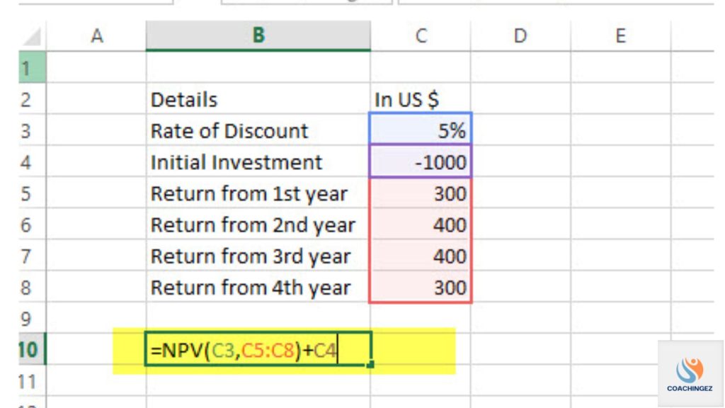
Financial Functions
6.1 PMT
PMT calculates the payment for a loan based on constant payments and a constant interest rate.
Formula:=PMT(interest_rate, number_of_periods, present_value)
Example:
For a loan with 5% interest over 10 years, =PMT(0.05/12, 10*12, -10000) calculates the monthly payment.
6.2 FV
FV calculates the future value of an investment based on periodic, constant payments.
Formula:=FV(interest_rate, number_of_periods, payment, present_value)
Example:
Returns the future value of an investment based on these variables.
6.3 NPV
NPV calculates the net present value of an investment based on a series of periodic cash flows and a discount rate.
Formula:=NPV(rate, cash_flow1, cash_flow2, ...)
Example:
Calculates the NPV for a series of cash flows discounted at a specified rate.
6.4 IRR
IRR calculates the internal rate of return for a series of cash flows.
Formula:=IRR(values)
Example:
This function returns the IRR for a series of investments.
7. Tips for Maximizing Efficiency with Excel Functions
- Use Named Ranges: Assign names to ranges so they’re easier to reference in formulas.
- Combine Functions: Many powerful formulas come from combining multiple functions.
- Utilize Keyboard Shortcuts: Excel offers shortcuts for common tasks (e.g.,
Ctrl + Shift + Lto toggle filters). - Practice Conditional Formatting: Apply formatting rules to quickly visualize data patterns.
- Use PivotTables for Summarization: PivotTables make large data sets more manageable and provide a flexible summary tool.
The Excel Functions Cheat Sheet from CoachingEZ is your go-to resource for mastering key Excel formulas such as SUM, IF, and VLOOKUP. With this guide, you’ll quickly learn how to streamline data processing, enhance accuracy, and boost productivity. Follow CoachingEZ to unlock powerful tips and become an Excel expert!
